why the words in “CAP theorem” are confusing

lets go through each one ok? my goal is to make you as confused as i am

consistency

the word “consistency” is super overloaded in the realm of distributed systems. In CAP, consistency means (informally) that every read reflects the most recent write. This is also known as single-copy consistency or strict / strong consistency. Data is replicated to multiple nodes in these systems, but any reads to this storage system should give the illusion that read and writes are actually going to the same node in a multi-user / concurrent environment. Put another way – there’s multiple copies of data in practice, but readers always see the latest (single) copy by some loose definition of “latest”.

unfortunately, “strong” consistency is a grey area with lots of informal definitions. Some distributed systems researchers such as Martin Kleppman equate CAP consistency with linearlizability, which depending on your definition of strong consistency, is either a weaker form of strong consistency or a more precise and formal definition of strong consistency. Does consistency mean that every write is instantaneously reflected on all nodes? Or, in the case of linearlizability, that even though reads may not reflect the latest write they will always reflect the correct ordering of writes based on some agreed upon global time?

data stores that support transactions are also characterized by their ACID properties (Atomic, Consistent, Isolated, Durable). ACID consistency has nothing to do with ensuring that readers get the latest write; ACID is about the preservation of invariants in the data itself (such as keeping debit or credit balanced) within a transaction, which is often the responsibility of the application itself rather than the storage system. Relational databases support specific forms of invariant enforcement through referential integrity, but many invariants cannot be easily enforced by the storage system. Are they related at all? Well, they’re related insofar as CAP consistency trade-offs affect ACID consistency for system designers, but they’re still completely different notions of consistency! For example, if it’s possible for a read to return stale data during a transaction (dirty reads), this can make it difficult to maintain invariants for the application.

availability

availability in CAP has very strict, binary definition. CAP availability states that every non-failing node (even if isolated from the rest of the system) can respond successfully to requests. This is confusing because most site operators talk about availability in terms of uptime and percentages. For example, consider this scenario of a system that currently serves most reads from secondary nodes. Lets assume that most secondary nodes in a system fails and can no longer serve requests. The server switches all reads to the primary and is still technically “available” from a user standpoint. This fails the CAP definition of availability, but passes the more practical operational definition of availability. One way to distinguish one from the other when they’re discussed at the same time is to refer to CAP availability as “big A” and practical availability / uptime as “little a”.

in practice, availability (“little a”) isn’t black and white (can EVERY non-failing node respond?). Most real world systems don’t even offer this strong guarantee. This definition might make sense in a theoretical system and make it easier to reason with more formally / mathematically, but in reality many storage systems allow users to choose between many different levels of availability and for different operations. For example, some databases allow users to tune availability by reads or writes using quorums. Systems that prioritize data durability in the face of failures may sacrifice some availability for writes. If writes cannot be propagated to a majority of nodes in the system, return an error. At the same time, it may also prioritize availability for reads and so perhaps any response from any replica is considered successful, even if that data might be stale. If you’re trying to reason about the availability of a storage system, these details matter and are far more relevant than whether or not the system is capable of achieving big A (CAP availability).

partition tolerance

partition tolerance is confusing on multiple levels.

the word “partition” itself is confusing because partitions in a distributed system are splits or shards of a data store that is maintained for purposes of scalability. In CAP, a partition refers to some network partition which is basically a network error that disrupts node to node communication. if a system remains operational in the presence of a network partition, then it is considered partition tolerant in the CAP model.

second, CAP appears to present partition tolerance as something a distributed system has or does not have. but because networks are fundamentally unreliable, system designers need to design systems to tolerate network errors. there’s not a really a choice or trade-off that should be made – it’s more of a requirement. unlike availability and consistency (which are actual trade-offs that need to be made when there is a network partition), partition tolerance is not something you can relax in practice. so designers are really choosing between consistency and availability, assuming that there will be network partitions. this is why some people say CAP is really just CP and AP. you’re either choose consistency with partition tolerance or availability with partition tolerance.

finally, partitions in the network are relatively rare events. two data centers or nodes within a data center may lose communication, but that’s rare compared to individual node failures (disk full, over-capacity, random crashes) that happen all the time given a large network. In the model of CAP, however, a single node failure isn’t a network failure and so it falls outside the stated rules of CAP. eric brewer has clarified though that in practice, nodes that fail to respond within some time window can be treated as conceptually equivalent to an actual partition event..

SICP Exercise 1.11 – Recursive & Iterative

Prompt

A function f is defined by the rule that f(n) = n if n < 3 and f(n)=f(n-1) + 2*f(n-2) + 3*f(n-3) if n >= 3. Write a procedure that computes f by means of a recursive process. Write a procedure that computes f by means of an iterative process. Hint: for iteration, think about how you might code this using a for-loop in a language like Python.

Solution

The recursive form is easier to tackle – LISP’s probably do the best job of expressing recursive mathematical expressions due to the extremely minimal syntax.

(define (fn n)
  (if (< n 3)
      n
      (+
       (fn (- n 1))
       (* 2 (fn (- n 2)))
       (* 3 (fn ( - n 3)))
      ) 
   )
)

Here’s an (incomplete) expansion using substitution of a call to (fn 10). Each newline denotes the expanded expression of the previous. Note the crazy combinatoric explosion of having not one but three recursive calls in the body – this creates a huge tree of deferred addition and multiplication operations.

(fn 10)

(+ (fn 9) (fn 8) (fn 7))

(+
 (+ (fn 8) (fn 7) (fn 6))
 (+ (fn 7) (fn 6) (fn 5))
 (+ (fn 6) (fn 5) (fn 4)))

(+
 (+
  (+
   (+ (fn 7) (fn 6) (fn 5))
   (+ (fn 6) (fn 5) (fn 4))
   (+ (fn 5) (fn 4) (fn 3))
  )
  (+
   (+ (fn 6) (fn 5) (fn 4))
   (+ (fn 5) (fn 4) (fn 3))
   (+ (fn 4) (fn 3) (fn 2))
  )
  (+
   (+ (fn 5) (fn 4) (fn 3))
   (+ (fn 4) (fn 3) (fn 2))
   (+ (fn 3) (fn 2) (fn 1))
  )
 )
 (+
  (+
   (+ (fn 6) (fn 5) (fn 4))
   (+ (fn 5) (fn 4) (fn 3))
   (+ (fn 4) (fn 3) (fn 2))
  )
  (+
   (+ (fn 5) (fn 4) (fn 3))
   (+ (fn 4) (fn 3) (fn 2))
   (+ (fn 3) (fn 2) (fn 1))
  )
  (+
   (+ (fn 4) (fn 3) (fn 2))
   (+ (fn 3) (fn 2) (fn 1))
   (+ (fn 2) (fn 1) (fn 0))
  )
 )
 (+
  (+
   (+ (fn 6) (fn 5) (fn 4))
   (+ (fn 5) (fn 4) (fn 3))
   (+ (fn 4) (fn 3) (fn 2))
  )
  (+
   (+ (fn 5) (fn 4) (fn 3))
   (+ (fn 4) (fn 3) (fn 2))
   (+ (fn 3) (fn 2) (fn 1))
  )
  (+
   (+ (fn 4) (fn 3) (fn 2))
   (+ (fn 3) (fn 2) (fn 1))
   (+ (fn 2) (fn 1) (fn 0))
  )
 )
)
...

Eventually, this long recursive process bottoms out at the base case when we reach (fn 2), (fn 1), and (fn 0) since none of those invocations will reach the recursive section of the procedure. For example, (fn 2) will return 2 since 2 < 3. These values will play an important role in developing the iterative solution.

Iterative Form

There’s a few ways to think about this problem to get an intuition about what the iterative form might look like. One way is to consider a similar problem such as the fibonacci sequence.

Fibonacci Sequence

Consider a similar mathematical expression such as the fibonacci sequence expressed in scheme as a recursive procedure.

(define (fib n)
  (if (< n 3)
      1
      (+ (fib (- n 1)) (fib (- n 2)))))

It’s simpler since there aren’t additional multiplication operations and you’re only dealing with two recursive procedures in the body instead of 3, but it exhibits the same pattern of process growth (exponential expansion followed by contraction).

(fib 5)

(+ (fib 4) (fib 3))

(+ (+ (fib 3) (fib 2)) (fib 3))

(+ (+ (+ (fib 2) (fib 1)) (fib 2)) (fib 3))

...

In the iterative form, you compute the next result using two values you currently have. You accumulate the answer from bottom up.

Here’s an example in scheme:

(define (fn n)
  (define (iter x a b)
    (if (> x n)
        a
        (iter (+ x 1) b (+ a b))))
  (if (< n 2) 1 (iter 2 1 1)))

a represents n - 2 and b represents n - 1. If we’re dealing with an n that’s less than 2, return 1. Otherwise kick off the recursive process with (iter 2 1 1). In each step, we compute the next result (+ a b) and feed that into our next recursive call as the new b.

There’s a few key insights from this iterative fibonacci definition:

  1. You start with two values and you use them to compute the next value. As the computation evolves, so do the two values you’re holding at any given point.
  2. Each step contains all the state you need to compute the next recursive step – there are no deferred operations
  3. Some notion of a “base case” is still necessary for knowing when to stop the accumulation. In this example we use x and we stop when x is greater than the initial argument to the fibonacci function.

Back to the problem

The fibonacci definition has a key trait in common with our problem. The current result based on n is based on computation using the last three results (instead of the two by fibonacci). In fact, they’re so similar that if you squint you might see the iterative form of our problem!

(define (fn n)
  (define (iter x a b c)
    (if (> x n)
        c
        (iter (+ x 1) b c (+ (* 3 a) (* 2 b) c))))
  (if (< n 3) n (iter 3 0 1 2)))

Unlike our fibonacci problem, we need to perform both addition and multiplication (+ (* 3 a) (* 2 b) c) in order to generate the next result. This is what moves the computation along. With fibonacci, there’s just an addition (+ a b) that gets computed as the new next value – but the same underlying pattern applies. Compute the next value, shift all three numbers forward and repeat.

Commentary

We got this problem on the first day of David Beazley’s SICP course and it completely destroyed my brain when I initially attempted to come up with the iterative solution to this.

The new syntax combined with the noise from all the additional computation in the recursive function made it very challenging. I didn’t really have an AHA moment to this until David shared his solution with us and I only realized the connection to fibonacci when I set out to write this post and revisit my understanding of the exercise.

I think this is a great problem in terms of noticing this tension between simplicity and beauty of recursive procedure definitions and their performance. You have this simple definition that grows wildly during runtime. Then you go forth and optimize it so that it doesn’t accumulate on the stack but get a far less intuitive looking definition as a result. There’s also the fun challenge of porting a recursive definition to an iterative one and noticing some of the difficulties in coming up with the right base cases. It’s really easy to make off by one errors with these problems and it’s not immediately obvious why the results are wrong until you go back to trace the mathematical definitions manually which can be tedious.

SICP Exercise 1.9 – Process Illustration

Prompt

Each of the following two procedures defines a method for adding two positive integers in terms of the procedures inc, which increments its argument by 1, and dec, which decrements its argument by 1

(define (inc x) (+ x 1))
(define (dec x) (- x 1))

; Implementation 1
(define (plus-v1 a b)
  (if (= a 0) 
      b 
      (inc (plus-v1 (dec a) b))))

; Implementation 2
(define (plus-v2 a b)
  (if (= a 0) 
      b 
      (plus-v2 (dec a) (inc b))))

Using the substitution model, illustrate the process generated by each procedure in evaluating (plus-v1 4 5) and (plus-v2 4 5). Are these processes iterative or recursive?

Solution

An important distinction to reiterate here is the difference between a recursive procedure and a recursive process. A procedure that references itself is a recursive procedure. In the implementations of plus above, both procedures are recursive. It’s a static construct. But a recursive procedure, at runtime, can generate an iterative process! Whether a process is iterative or recursive depends on the manner in which the computation is carried out.

A common way to illustrate each evaluation step of a procedure application process is using the substitution model to show the expression that gets evaluated.

Here’s an example of using substitution applied to the first plus procedure.

(plus-v1 3 5)
(inc (plus-v1 2 5))
(inc (inc (plus-v1 1 5)))
(inc (inc (inc (plus-v1 0 5))))
(inc (inc (inc 5)))
(inc (inc (+ 5 1)))
(inc (inc 6))
(inc (+ 6 1))
(inc 7)
(+ 7 1)
8

The first (plus-v1 3 5) expression is our initial procedure invocation.

If we evaluate this we will get our next result. Since 3 does not equal 0, the if statement is skipped and we get (inc (plus-v1 2 5)). If we evaluate this again, notice that we don’t expand the expression for inc yet because we don’t know what the value of it’s argument is. We need to continue expanding the plus expressions until we reach an actual primitive value.

In other words, we are deferring the evaluation of inc until later. If you look at our full expansion, we only start calling inc when we get the value 5 back from (plus-v1 0 5). This chain of deferred operations during the evaluation process makes this a recursive process!

Now contrast this to the other plus procedure plus-v2.

(plus-v2 3 5)
(plus-v2 2 6)
(plus-v2 1 7)
(plus-v2 0 8)
8

In each step of the evaluation, no operation is deferred. We’re incrementing one number, decrementing the other and calling the function again. There are no function calls waiting for a result. This is an iterative process. In iterative processes, the complete state is computed in each step. In other words, prior to calling the procedure, all the parameters that would bind to the arguments are provided with primitive values.

Comments

When we did this exercise with David Beazley in his SICP course, he joked that this exercise was sort of like desert island coding. You’re stranded on a desert island… if you only had increment and decrement, how would you add addition and multiplication? Funny enough, he was actually stuck in a scenario not too far from that when he had to re-invent the shell using python while locked in a secure vault (very entertaining talk!).

What I like about this exercise is how effectively it gives students a feel for the difference between recursive and iterative processes. By expanding out an expression by hand using substitution, you can see operations expanding and contracting. This raises a lot of interesting ideas and questions around performance, recursive function base-cases, and whether all recursive forms have an iterative form and vice-versa.

SICP Exercise 1.6 – Cond as If?

Prompt

Alyssa P. Hacker doesn’t see why if needs to be provided as a special form. “Why can’t I just define it as an ordinary procedure in terms of cond” she asks. Alyssa’s friend Eva Lu Ator claims this can indeed be done, and she defines a new version of if:

(define (new-if predicate 
                then-clause 
                else-clause)
  (cond (predicate then-clause)
        (else else-clause)))

Eva demonstrates the program for Alyssa:

(new-if (= 2 3) 0 5)
5
(new-if (= 1 1) 0 5)
0

Delighted, Alyssa uses new-if to rewrite the square-root program:

(define (sqrt-iter guess x)
  (new-if (good-enough? guess x)
          guess
          (sqrt-iter (improve guess x) x)))

What happens when Alyssa attempts to use this to compute square roots? Explain.

Solution

The new-if appears to work since in the simple example we’re getting the correct results. However, the applicative order of evaluation of the new-if is a subtle but important difference compared to the actual if statement.

With applicative order evaluation of function applications, both the then-clause and the else-clause gets executed. We’re going to end up always evaluating sqrt-iter even if the guess is good enough. This completely breaks recursive procedures that rely on the satisfaction of base case conditions to terminate calls. In this case, the recursive calls will never end because sqrt-iter will be called all the time.

I really like this exercise because at a glance, it seems perfectly reasonable to implement if in terms of cond – I mean, they both exhibit the evaluation style that you want. else clauses won’t be executed at all if the predicate is true. So why not just substitute one for the other?! That sounds good! But in trying to do this by defining a new function, you immediately lose the special-case evaluation behavior 😹. This really further drives home the essential nature of lazy evaluation behavior for conditionals.

I think often as consumers of programming languages we take this behavior for granted and don’t think twice about how conditional expressions are evaluated. But this sort of exercise (and many exercises in SICP!) puts you in the seat of the language designer.

Difference between Docker ENTRYPOINT and CMD

ENTRYPOINT and CMD are two docker commands that sound interchangeable, but there are important differences that I’ll cover in this post. I suspect CMD is probably the more familiar instruction, so I’ll go over what that does and how it differs from ENTRYPOINT.

Here’s the purpose of CMD, taken straight from the docker manual:

The main purpose of a CMD is to provide defaults for an executing container.

https://docs.docker.com/engine/reference/builder/#cmd

If you start a container via docker run or docker start and you don’t supply any commands, the last CMD instruction is what gets executed. In most docker files, this effectively acts as “main” or … “entrypoint”. I put entrypoint in quotes both to distinguish it from the formal ENTRYPOINT instruction and to show you why this naming is confusing!

Here’s an example of a dockerfile that runs the rails server using CMD

# Use a base image with Ruby and Rails pre-installed
FROM ruby:3.2

# Set the working directory inside the container
WORKDIR /app

# Copy the Gemfile and Gemfile.lock to the working directory
COPY Gemfile Gemfile.lock ./

# Install dependencies
RUN bundle install

# Copy the rest of the application code to the working directory
COPY . .

# Set the default command to run the Rails server
CMD ["rails", "server", "-b", "0.0.0.0"]

CMD does not create a new image layer, unlike commands like RUN. It does not do anything at build time. So when you run docker build to create a docker image from a dockerfile, rails server is not being executed. It purely a runtime (container runtime) construct. This interleaving of instructions in docker that are intended for difference stages of a container lifecycle is also a common source of confusion for beginner users of docker.

In practice, at least from my experience, CMD is sufficient. I work on mostly web services and the vast majority of containers are running a server process of some kind using CMD <start server> after the application dependencies are build. For most situations, this is enough and you never have to think about or even be aware of the existence of ENTRYPOINT.

Have a nice day.

Just kidding, okay lets go over ENTRYPOINT now.

Here’s a rather confusing description on dockers website on what ENTRYPOINT is:

An ENTRYPOINT allows you to configure a container that will run as an executable.

https://docs.docker.com/engine/reference/builder/#entrypoint

So CMD is to provide defaults for an executing container and ENTRYPOINT is to configure a container that will run as an executable. That’s a little confusing because using CMD sort of also allows you to run a container as an executable right? You start the container and something executes!

Here’s a simpler definition:

An ENTRYPOINT is always run. It doesn’t matter what arguments you’re passing when running docker run. ENTRYPOINT is never overwritten. If arguments are passed, those are appended to the end of what’s already specified in ENTRYPOINT.

Here’s an example of using the ENTRYPOINT instruction in a Dockerfile:

FROM ubuntu:latest
ENTRYPOINT ["echo", "Hello, World!"]

In this example, the ENTRYPOINT is set to the command echo "Hello, World!". When a container is created from this image and started, the message “Hello, World!” will be printed to the console. Running docker run my-image "Welcome" would result in the message “Hello, World! Welcome” being printed.

Let’s take a look at an example using CMD to demonstrate the override behavior:

FROM ubuntu:latest
CMD ["echo", "Hello, World!"]

In this case, the CMD instruction specifies the default command as echo "Hello, World!". However, if a user runs the container with a different command, the specified command will override the CMD instruction. For instance, running docker run my-image "Welcome" would output “Welcome” instead of the default message “Hello, World!”. The entire command is overridden.

Both CMD and ENTRYPOINT can be used together in situations where you want

  • A particular command to always execute (this is where ENTRYPOINT comes in handy) that cannot be overridden
  • A set of default arguments for the ENTRYPOINT command

This offers some flexibility in how users of your image can provide custom arguments to alter the runtime behavior of your container. In cases where you don’t need that customization or where it’s perfectly fine for users to provide their own “entrypoints”, just use CMD.

Distributed Caching Pattern: Write Through

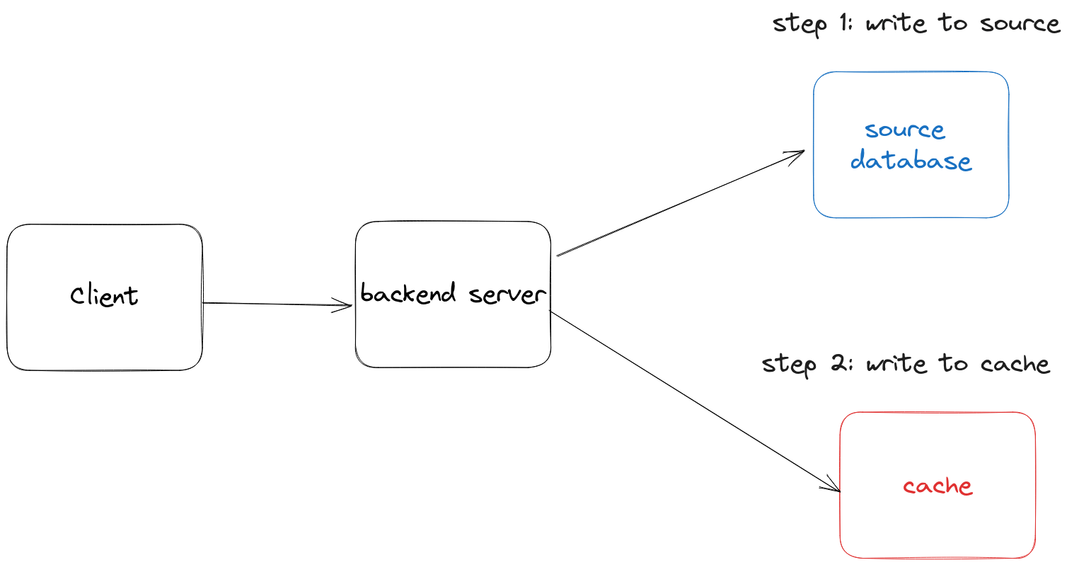
Write-through caching is a caching mechanism where data modifications are written to both the source database and the cache. In this approach, every write operation triggers a write to a RAM cache (such as redis) and the source database (such as postgres).

This is commonly used to complement look-aside caching pattern so that when subsequent read operations request the same data, there’s a greater likelihood of a cache-hit, therefore reducing the response time and minimizing the load on the source data store. Additionally, the cached data being returned will be more fresh compared to a strategy that only uses TTL or expiration based invalidation.

The key benefit to using a write-through cache is data freshness. By updating the cache during updates to the source database, you ensure that the cached data remains up to date. One of the common problems with relying strictly on expiry based invalidation to serve fresh data is the risk of stale data during the period between when the data is cached and when it expires.

How to implement (Ruby on Rails Example)

Lets look at a simple example. When data needs to be written, it is first updated in the source database and then persisted in the cache. Here’s an example using rails. In this example, we’re reading a list of blog posts using look-aside caching. On writes (updates to an individual blog post), we update the cache. This keeps the list of blog posts in the cache fresh!

class PostsController < ApplicationController
  def index
    @posts = Rails.cache.fetch('posts', expires_in: 1.hour) do
      Post.all.to_a
    end
    render json: @posts
  end

  def create
    @post = Post.new(post_params)
    if @post.save
      update_posts_cache
      render json: @post, status: :created
    else
      render json: @post.errors, status: :unprocessable_entity
    end
  end

  def update
    @post = Post.find(params[:id])
    if @post.update(post_params)
      update_posts_cache
      render json: @post
    else
      render json: @post.errors, status: :unprocessable_entity
    end
  end

  def destroy
    @post = Post.find(params[:id])
    @post.destroy
    update_posts_cache
    head :no_content
  end

  private

  def post_params
    params.require(:post).permit(:title, :content)
  end

  def update_posts_cache
    Rails.cache.write('posts', Post.all.to_a, expires_in: 1.hour)
  end
end

In this example, the index action retrieves the list of blog posts from the cache using the key `posts`. If the cache contains the posts, they are returned directly. Otherwise, the posts are fetched from the database (Post.all.to_a) and stored in the cache with a 1-hour expiration time.

Implementing write-through isn’t always straightforward because cached data may not always be easily re-computed on writes. The extent to which you can re-compute cached data during a write greatly affects the feasibility of a write-through implementation. In the example above, we re-computed the list of posts in the cache by invoking Posts.all.to_a in the code for writing. But what if instead of serving all posts on reads, our application only serves unread posts for logged in users? If you have 10 logged in users, they need to be served different lists of posts! (As an exercise, think about how you would handle this!).

Sometimes cache re-computability is affected by the API paradigm you choose. RESTful services are able to leverage write through caching better than GraphQL services. Lets see why.

GraphQL and Write Through Caching

At work we heavily use GraphQL API’s and GraphQL presents unique challenges for caching. The entire paradigm of GraphQL rests on allowing clients to query for the data they need. This leads to a higher variability in queries of nearly unbounded complexity (you can have highly nested queries). Common caching techniques can be easily applied to applications serving a small set of frequently executed but fixed queries – but if every query is likely going to be unique, the value of caching is diminished.

There’s a bigger reason though why caching (particularly write-through caching) is trickier with GraphQL. In reality, most GraphQL servers are built for internal product teams and client queries aren’t infinitely variable. There’s typically some fixed number of clients that use some set of queries to power an experience.

For example, at a video streaming company there may be a recommendations team (the client) that uses a set of queries for fetching video metadata from an internal video catalog service (graphql server).

Lets assume…

  1. There’s a high traffic query that looks like this defined within the recommendation client: query { videos { title createdAt reviews { reviewerFullName } } }.
  2. Within the video service, query results are cached on read with look-aside caching.

Now lets say you want to implement write-through caching to keep the cache of the recommendation teams query results warm. If video metadata gets updated throughout the day in the video catalog service (lets just say by some other service via HTTP), how does the cache get updated?

Here’s what we know:

  1. The query is defined on the client (unlike REST, where the query is defined on the server).
  2. The result of the query operation is computed at runtime in the video service resolvers.

This is a situation where the cached data (JSON result of the GraphQL query) is no longer easily computable. In order to compute that data, you need to execute the original query against the schema using the same inputs. But wait, GraphQL servers don’t define the queries, clients do! 😞

Unless the application changes the type of data that gets cached or the server records queries being executed against the API (to be “replayed” on relevant writes), warming this type of cache using write-through is not really possible. So in practice, most GraphQL servers focus on lazy-loading read-based caching strategies such as automatic persisted queries using GET requests or fragment caching on the server side.

Risks

Adopting write-through caching isn’t without risks – before implementing it, it’s worth considering the following in the context of your unique problem.

  • Increased Write Latency. Write-through caching introduces additional overhead due to the need to write data to both the cache and the main data store before returning a result. This can be an issue for applications with high writes that cannot tolerate additional write latency. That said, most users of applications generally have higher tolerance for writes than for reads.
  • Redundant / Unnecessary data in cache. The cache may fill up regardless of whether the data being written is going to be used. Data being written isn’t really a guarantee of a future read, so you may end up with a cache filled with unread data (which defeats the purpose of a cache). If you don’t have proper eviction policies in place, systems with high write volumes with large amounts of data being written can rapidly fill up a cache and make it unusable. On the other hand, if there are eviction policies in place and you haven’t properly sized your cache, you end up with churn in your cache where data being written to the cache is evicted before it has a chance to be used by readers.
  • Delayed benefit. The cache is only updated when something changes as a result of a write. If nothing changes, the cache stays empty. This is also why you rarely see systems that rely exclusively on write-through caching. If updates are infrequent, the cache will stay cold forever unless you also cache when the data is being read.

Questions to ask before caching with a remote cache

Distributed caching with a system like memcached or redis comes at a cost! If you haven’t added a remote cache yet, here’s some costs to consider:

  1. The operational cost of actually standing up and maintaining a remote caching service. Is it a managed service like AWS elasticache or self managed? What are the failure modes? How does it get secured and upgraded?
  2. More complexity in having another system in the call stack that makes it harder to understand and troubleshoot application behavior. Data freshness and consistency issues come to the forefront whenever a cache (or really any derived data) is involved.
  3. General exposure to a entire class of new problems (cascading failures) that comes with sharing load with another system.

Even if you already operate or use a remote cache, caching any bit of data still adds complexity to your application – and not the essential kind. It’s easy to use caching strategies as a hammer for every performance issue, but here are some questions I recommend you ask before reaching for caching as a solution.

Have I figured out what the problem really is? Is speed really an issue?

Programmers tend to want everything to be fast – and while it’s important that apps generally feel snappy and help users get stuff done efficiently, speed doesn’t impact the user experience the same way in every interaction they have with your app.

For example, users expect fast read experiences (like searching a catalog on ecommerce sites) but slower write / update experiences (like submitting a payment). If you spend all your time optimizing a slow payment submit process when most of your users are bouncing because they can’t be bothered to even look at your inventory, you’re wasting your time.

What specifically needs to be faster and by how much?

Just like most metrics, optimization has diminishing returns. How fast do you want an experience to be? Under a second? Under 100 milliseconds? If your p99 is < 100ms and there’s no reason to believe that your users are unhappy with performance, the return on investing time in reducing latency may be low.

The marginal value of optimization depends on your use-case and current baseline performance. If you’re a backend API team with an SLA, the specific numbers may even be hard coded into a contract. If there are no binding agreements on performance, the requirements are fuzzier and may be driven more by best practices and customer reports. In either case, do some cost benefit analysis – this doesn’t have to be rigorous and sometimes the reason to do it regardless of how high the lift is may be as simple as “users will stop using this dashboard if it continues taking five seconds to load”.

Finally, once you’ve picked a target don’t forget to measure your performance progress. Are there certain metrics (percentile latency, profiling stats, etc) you can use to describe the current performance and how will you know when you’ve reached your goal? I really enjoy performance work, but I also know I need to know when to stop at the risk of losing sight of other goals.

Can I optimize without caching?

Reaching for caching as a strategy in a first pass at performance work does two things that are not ideal for the resilience of your system.

  1. It hides inefficiencies (poorly written queries, N^2 algorithms) that exist in your program that will be much more difficult to spot once the cache is in place.
  2. It can make your cache load bearing over time, meaning unless your cache is healthy, your application is unusable under normal load. Since most distributed in-memory caches are, by design, meant to be volatile and ephemeral, cold-cache events become an Achilles heel for your system.

Before you cache data, consider common performance bottlenecks in your system. Some common examples for web apps are:

  • Excess database querying such as N+1 queries.
  • Excess memory allocation, especially for garbage collected languages. I currently use rails for word and Active Record object allocations are particularly expensive since they lead to longer GC cycles that impact latency.
  • Missing HTTP response compression (gzip compression for example at a reverse proxy).
  • In-efficient algorithms, such as slow compute inside nested loops. Worth knowing the basics of Big O here.

Can I cache outside of my origin server?

Ok, so you need to cache – but can you cache the data such that:

  1. The data is as close to the requester as possible, therefore much faster to serve!
  2. Your backend server can sit back and do zero work (isn’t that great?)

The good news for web applications is that browser clients have their own cache. By using proper cache-control HTTP headers, you can have control over what requests are cached and for how long. If the data is too dynamic (unique to individual users for example) to cache for any length of time, consider if you can make it static (same for all users). If you can’t make it static, can you extract the parts that are static and cache that?

Most enterprise applications with global customer bases also make use of Content Delivery Networks (CDN’s) that have points of presence (data centers strategically located in geographic locations around the world) that can serve requests out of its own cache without reaching to the origin servers.

Delegating caching behavior to systems closer to your clients isn’t a mutually exclusive strategy to caching at origins with remote in-memory systems, but they can be a low effort (implementation wise) and significantly faster caching approach so they’re worth trying out first if they’re not being used.

Forward Proxy vs Reverse Proxy

Two main types of proxies are forward proxies and reverse proxies. Since they’re both proxies, it’s not immediately obvious from their names how they’re different! All proxies act as a middle man in a network topology between two parties: the client (or thing requesting a resource) and a server (the thing providing the resource).

The proxy itself is technically also a server, but in most discussions / writing about proxies the “server” is referring to the server that is providing the resource (such as an HTML page) that the client is requesting. If you’re running a web service, that server would be the backend service such as a rails app.

Forward Proxy

A forward proxy is a proxy that clients connect directly to and is aware of. The proxy itself is not aware of backend server identities / IP’s – it only knows how to forward and respond to requests. The client knows that its connecting to a proxy – and by client I don’t mean the actual computer user, but rather the program (perhaps a browser) that’s connecting to the wider internet. Sometimes the real user doesn’t even know that there is a proxy involved!

Here’s a couple of real scenarios involving forwarding proxies:

  1. A VPN service that clients can connect to hide their origin IP’s for the sake of protecting their identity (maybe for the purposes of bypassing censorship or just to remain anonymous). VPN’s are a special type of forwarding proxy that provides additional security and authentication features for the purposes of protecting the anonymity of the client requesting a resource. Since users are the ones seeking protection when signing up for VPN services, they’re also aware that the system they’re using is making use of a proxy server.
  2. A firewall proxy setup by school network administrators to intercept and block traffic to and from certain sites (social media sites, porn sites, etc). In this situation the computer user may be unaware that they’re being restricted – a student tries to access a restricted site and find it blocked, unaware that the client programs on their computer are configured to connect to a firewall proxy that is snooping on their requests.

Reverse Proxy

A reverse proxy is one that client programs are not aware of. Additionally, the proxy itself is aware of backend servers.

Clients have no idea that they’re connecting a reverse proxy. For example, so much of the internet services you use day to day sit behind reverse proxies – but I’m sure you have not configured your programs to connect to each one of these reverse proxy servers. Even though requests from clients are reaching the reverse proxy servers just like forwarding proxies, the clients do not actually know that they’re proxies.

On the other hand, the reverse proxy is aware of backend servers. It accepts incoming requests from clients and then forwards them to specific servers.

A few of the most common scenarios involving reverse proxies are:

  1. To improve the reliability of a service by load balancing traffic between backend servers. Nginx is a popular reverse proxy used by some of the biggest sites in the world. If you’re a developer, you can set up nginx in front of your application servers and have distributed traffic using algorithms like round robin or least time.
  2. To improve the security of a service by acting as the single authentication point for things like TLS handling / TLS termination and protecting the actual IP’s of your backend servers.
  3. To improve the performance of a service by compressing outbound traffic so that reducing response sizes to clients as well as caching static files so that requests for the same files such as images don’t need to go directly to your backend servers.

To sum it up – a forward proxy is cooperating with the clients to help the clients achieve X (bypass firewalls or in the case of firewall proxies to impose limitations). A reverse proxy is cooperating with servers / backend servers to achieve X (service reliability, security, etc).

Distributed Caching Pattern: Cache Aside

A distributed cache is a remote caching system that an application uses via a network to reduce read latency. There are lots of ways an application can interact with this cache and there tends to be common access patterns or strategies – one of the most popular access pattern is called “Cache Aside” (sometimes also referred to as look-aside or lazy load) and I’ll cover both the benefits and risks of this pattern in the context of a web app.

In a cache-aside, the application is able to connect to both the cache store and the source store (this is typically the primary, higher engine latency data store). If the application is a web application, the way this pattern works is:

  1. App receives a request for data.
  2. App looks up the data in the cache. If it’s in the cache (cache-hit), return it. If not (cache-miss), fetch the data from the source.

As with any caching pattern, the usefulness of a cache is influenced by how much faster it is to access the same copy of data from the cache compared to the source and the cache hit ratio (also known as the hit ratio or hit rate).

A cache hit ratio is the percentage of total requests to the application that results in a cache hit (number of cache hits / (number of cache hits + number of cache misses)). If you have a cache hit ratio of 1, that means every request resulted in a cache hit. If you have a cache hit ratio of 0, that means no requests resulted in a cache hit.

Pros and Cons

Here are some advantages or benefits to using a cache-aside pattern:

  • It’s relatively straightforward to implement once you’ve identified what you want to cache. In most cases this involves adding a single new line of code to perform the lookup in the cache before executing the original source store lookup. As a maintainer of that code, it’s also easier to reason with since the caching decision is made explicit in the source code.
  • You’re more likely to cache data that is going to be requested multiple times because you’re always caching by demand. The cache store is only populated whenever there is a cache-miss, so you’re more likely to cache the data you actually want cached and the storage footprint is lower.
  • Since you’re caching on demand, you can start benefiting from this cache pattern immediately once it’s in place because the cache will naturally fill up overtime without requiring any sort of offline cache pre-population.
  • In the event of a cache fail-over event, there’s a natural fallback already in place in your application (hitting the source database). In other words, since the application knows how to connect to both data stores, there’s a built-in redundancy which makes it more resilient to caching system failures.

Risks or things to watch out for with this pattern:

  • Since we’re only caching on demand, there will always be a cache-miss for initial requests. This might be bad if the cost of a cache miss is very high (lets say it involves some heavy compute that will cause potential customers to your site to bounce). When there’s high load, you’re also susceptible to a cache stampede.
  • Cache-invalidation is something you still need to reason about since this pattern has zero say / opinion on how data stays fresh once it’s stored for the first time. How long does it stay in the cache (TTL) ? What are the requirements around data freshness? If the underlying data is something that changes often (lets say it’s a list of book recommendations that gets pre-computed offline), how do you push those changes to the cache if at all? These are generally important questions to ask regardless of what caching pattern you’re using, but they’re especially critical when you’re using this particular pattern.
  • It’s very easy for the cache to become load-bearing overtime. If an app cannot adequately service it’s normal levels of traffic without the cache, the cache is load bearing. This isn’t great because it means that the cache becomes a single point of failure for your business and this dependence creeps up with this particular caching pattern because it’s easy to ignore the real costs of data access once you’re serving the majority of your traffic via the cache.

On cache hit ratios

The cache hit ratio alone doesn’t say much about the usefulness of a cache.

What you’ll typically notice with this pattern is that the hit rate starts out very low (on a cold cache) and then gradually increases as more data is cached until it stabilizes. If you’ve just restarted your cache and it’s cold, having a hit rate of 0 for the first say 10 minutes doesn’t tell you much about the effectiveness of the caching pattern if eventually the hit rate rises and stabilizes at a satisfactory level.

Traffic patterns can also affect your cache – if you’re experiencing a period of low variability in queries, your hit rate is going to be high during that period which may be misleading if during normal periods of traffic you get a much wider distribution of unique requests that are likely to miss your cache.

Lastly, if your hit rate is high, it really only tells you that your cache is working but not whether it’s actually working better than the actual un-cached path. Long story short – it’s a data point, but don’t take it as gospel and look at it in context of your entire application.

Newtons Square Root Method in Racket

Isaac Newton came up with an elegant method for calculating square roots through a series of approximations that get refined over time. At the end of this post, I will show a racket implementation of the procedure.

Overview

The square of \(x\) can be written as either \(2*2\) or in the exponential form \(x^2\). Therefore, the square of 2 is 4 because \(2*2\) is 4 and the square of 3 is 9 because \(3 * 3\) is 9. It’s called squaring because when you multiply a number by itself, you form the area of a square since the two numbers are the same and can be conceptualized as equal sides on a square.

Square roots are the inverse of squares and the square root of x can be written in its fractional exponential form \(x ^ {1/2}\) or more commonly \(\sqrt{x}\). If \(\sqrt{x} = y\), then it must also follow that \(y^2 = x\).

A perfect square is a number that is the product of a number multiplied by itself. Some examples of perfect squares are 4 (\(2*2\)), 9 (\(3*3\)), 16 (\(4*4\)), and 25 (\(5*5\)).

Finding the square root by … guessing

What’s the square root of 9? How do you compute this in your head if you don’t already know that the answer is 3?

Start guessing!

Pick a number less than 9 and square it and see how close I get to 9. If the answer is less than 9, then the square root must be larger than my current guess. And if it’s larger than 9, then the square root is smaller than my current guess.

There’s two parts to this process:

  1. Guessing a number that represents the square root
  2. Checking whether the square if the guess is within the threshold of what we are looking for (as close to 0 as possible)

To phrase this more precisely, given \(\sqrt{x}\), we’re looking for \(y\) such that \(x – y ^ 2 = 0\).

A closer look at newtons method

\(let\ a = 9\), where 9 is the number we’re trying to find square root for. Think of it as the total area of a rectangle.

\(x\) is our guess.

\(y\) is the other side of our rectangle such as \(x*y = a\)

Think of 9 as an area of a rectangle. You can form it in different ways / different dimensions but with the same area. The last shape is a perfect square with equal sides – the side of a perfect square is what we’re looking for.

Given any \(x\) and \(y\) such that \(x * y = a\), we know that any other value less than \(x\) if \(y\) is unchanged will be < \(a\) and any value more than \(y\) will be > \(a\).

To make a better guess towards a value that brings us closer to the perfect square such that \(x * y = a\) and \(x = y\), \(x\) needs to be bigger and \(y\) needs to be smaller.

Basically, we want \(x\) to be as close to \(y\) as possible, so they need to get closer over time in order for us to find the answer. Therefore, a better guess needs to be a value that is between \(x\) and \(y\).

One such better guess is the average of \(x\) and \(y\)!

By repeating this process, we converge on the answer.

Racket Implementation

#lang racket

(define (sqrt x)
    (define (square x) (* x x))

    (define (good-enough? guess x)
      (< (abs (- (square guess) x)) 0.001))

    (define (average x y) (/ (+ x y) 2))

    (define (improve guess x)
      (average guess (/ x guess)))

    (define (sqrt-iter guess x)
      (if (good-enough? guess x)
          guess
          (sqrt-iter (improve guess x) x)))

    (sqrt-iter 1.0 x)
)

SICP Exercise 1.5 – Testing Evaluation Order

Prompt

Ben Bitdiddle has invented a test to determine whether the interpreter he is faced with is using applicative-order evaluation or normal-order evaluation.

To refresh your memory, “applicative-order” means that procedure arguments get evaluated before being substituted into a procedure. “Normal-order” means that procedure arguments get evaluated later and only if needed (lazy).

He defines the following two procedures:

(define (p) (p))

(define (test x y) 
  (if (= x 0) 
      0 
      y))

The first procedure is a function by the name p that returns the invocation of itself. So it’s a recursive call. The second procedure performs a conditional check on two variables. If x is zero, return zero. Otherwise return y.

Then he evaluates the expression

(test 0 (p))

What behavior will Ben observe with an interpreter that uses applicative-order evaluation? What behavior will he observe with an interpreter that uses normal-order evaluation?

Explain your answer. (Assume that the evaluation rule for the special form if is the same whether the interpreter is using normal or applicative order: The predicate expression is evaluated first, and the result determines whether to evaluate the consequent or the alternative expression.)

Solution

Consider applicative order first where arguments are evaluated first before being passed into the function.

Given (test 0 (p)), the arguments are 0 and (p).

0 is a literal primitive so it just evaluates to itself (zero).

(p) is a procedure application (a procedure that accepts no arguments) that returns the result of another procedure application (the application of itself, p). Since it’s an application that returns the application of itself with no terminating condition, it’ll continue applying itself indefinitely! In other words, we’ll never actually get a chance to enter into the test procedure call due to this non-terminating procedure.

On the other hand, with normal order evaluation where the arguments are evaluated on when needed, (test 0 (p)) will expand to (if (= 0 0) 0 (p)).

Since the condition is true, and given that the if special form never evaluates the right hand side expression unless the condition is false, the return value is 0. If we changed our procedure application to (test 1 (p)) however, it’ll enter into an infinite loop.

Takeaway

This small example demonstrates a fairly deep idea. Given the same arguments to a function and applying the substitution model of reasoning about how symbols get replaced with values, evaluation order matters. This is not an obvious concept and one that surprised me even though I’ve been programming for many years.

If most languages you’ve used implement applicative order evaluation, code that looks like should exhibit the same behavior in a language that uses normal order evaluation would be surprising.

What are the pros and cons of normal order evaluation?

Are there any programming languages that use normal order evaluation?

How do you implement normal order evaluation in an interpreter?

What’s the difference between controlled and uncontrolled inputs in ReactJS?

Uncontrolled inputs are input elements that have their state stored strictly in the browser document object model (DOM). They behave like vanilla HTML inputs that you create without using a framework like React.

Uncontrolled (out of control? lol) inputs

There’s a couple of ways you can create uncontrolled inputs.

The first is to leave out the value attribute of an input.

function App() {
  return (
    <div>
      <input type="text" name="title"/>
    </div>
  );
}

This input behaves like a regular input. But if you need to access the value of this input inside your component – say, to submit the form or to do some other processing with the value – then you can’t access it without directly accessing the value from the DOM itself using the DOM API (i.e document.getElementsByTagName).

If you’re using ReactJS in the first place, you’re probably trying to avoid having to work directly with the DOM API. Now there are situations when you do want to read DOM state directly and React offers a way to do that with uncontrolled inputs through its own API called refs.

Here’s an example of reading state from our uncontrolled component with refs:

App() {
  const inputRef = useRef(null);
  const handleClick = () => {
    alert(inputRef.current.value);
  };
  return (
    <div>
      <input type="text" name="title" ref={inputRef} />
      <button onClick={handleClick}>Click</button>
    </div>
  );
}

We bind the input to a ref object that’s created using the useRef hook. This creates a connection to our input element and allows us to access the DOM value directly without having to use the DOM API. In most situations where you want or need to use uncontrolled inputs, refs are the way to go.

You can also create an uncontrolled input by setting a value attribute – but only if the value is null or undefined.

Here’s an example with undefined

function App() {
  return (
    <div>
      <input type="text" name="title" value={undefined} />
    </div>
  );
}

This behaves just like an input that doesn’t have a value attribute at all.

Controlled inputs

Controlled inputs that get their value from React component state rather than from the DOM. The component is the source of truth for the value of the input.

For example

function App() {
  const [title, setTitle] = useState("dog day afternoon");
  return (
    <div>
      <input type="text" name="title" value={title} />
    </div>
  );
}

If you tried to type into this input, the value won’t actually change! That’s because nothing in the component is currently writing to the title variable. That’s why most controlled inputs will come with change handlers.

function App() {
  const [title, setTitle] = useState("dog day afternoon");
  return (
    <div>
      <input type="text" name="title" value={title} onChange={(e) => setTitle(e.target.value) }/>
    </div>
  );
}

Danger! Changing a controlled input to an uncontrolled input between renders

Now that we’ve covered the difference between a controlled and uncontrolled component – what happens if this same input element changes from a controlled element to an uncontrolled one?

To demonstrate what happens, lets add a toggle handler that toggles the title state between a string value and undefined.

function App() {
  const [title, setTitle] = useState("dog day afternoon");
  const toggleTitle = () => {
    if (title) {
      setTitle(undefined);
    } else {
      setTitle("dog day afternoon");
    }
  }
  return (
    <div>
      <input type="text" name="title" value={title} onChange={(e) => setTitle(e.target.value) }/>
      <button onClick={toggleTitle}>Toggle</button>
    </div>
  );
}

Clicking toggle produces the following error

Warning: A component is changing a controlled input to be uncontrolled. This is likely caused by the value changing from a defined to undefined, which should not happen. Decide between using a controlled or uncontrolled input element for the lifetime of the component. More info: https://reactjs.org/link/controlled-components

In most cases, you can fix this by ensuring that you don’t supply undefined or null to your inputs. You can do this with some additional data processing or validation before that value is bound to the input at render time.

Web Application Session Management Primer

Most web applications need to handle user sessions at some point. A common use-case is to remember an authenticated user across requests. Since HTTP is a stateless protocol, the only way for servers to know that the current request is related to a previous request by the same user is to associate them with some common identifier provided by the browser containing information about the user.

A popular and simple way that browser clients provide this identifier is to do it completely through cookies – this is also known as client side session management.

Here’s a typical scenario involving cookie sessions:

  1. User submits login credentials for web app
  2. Server authenticates the user credentials and asks the browser to set a cookie containing information (such as user ID) that allows the server to re-authenticate the user on subsequent requests
  3. After the cookie is set, the browser forwards cookies to the app as long as it’s active and not expired.
  4. The app reads the cookie and the user ID that the cookie contains and then performs a user lookup using the ID. If the user exists, they’re authenticated and the application can respond accordingly.

In most production systems, the cookie contents are typically masked and cryptographically signed so that they can’t tampered with. This is important because if cookie contents can be easily modified, any authenticated user can impersonate any other user just by changing the contents of the cookie like user_id.

Drawbacks of client side management

While a fully client side approach that’s easy to set up – and very secure if done right – there’s some drawbacks as well.

  • If your server keys are exposed, the contents of any cookie generated by the key can be tampered with. This can be bad if the cookies contain personally identifiable information (PII) or worse, user credentials.
  • You are reliant on the browser to expire user sessions since the entirety of session state lives in the browser. To get rid of a cookie, you need to make sure to set cookie expiry headers and wait for the browser to expire them. If cookies are being cryptographically signed, you can technically rotate your key to invalidate all sessions… but that’s a nuclear option.

The one-sided nature of an applications control over session life and potential for leaking sensitive information into the client leads many applications to adopt a server side session management – a different, more operationally expensive approach that comes with a different set of trade-offs.

Server Side Management

Server side session management (SSM) is a bit of a misnomer because session related data is not completely server side. Remember, HTTP is a stateless protocol – the only way for a remote server to tell that requests are related is from information passed along by the client.

SSM still uses cookies for session management, so what part of it is server side?

Instead of storing the actual contents of a session like user id (encrypted or not, doesn’t matter) directly in the cookie, it stores a reference to the data in the form of a session ID – also known as a session token. When the client makes a request to the web application, it forwards this cookie containing the session token and the application uses it to look up the actual contents.

With a server side approach, you can use cookies to persist a common session state without risk of exposing data on the cookie itself since the actual data is stored server side. You can… have your cookie and eat it too.

Okay, so where is the actual content stored?

The two primary locations for session contents are either on same application servers receiving requests or in a database running on another server.

Storing session data on application servers

The easiest option is on the application server itself, either on disk or in memory. On a single server setup, sessions will go down with the server if in memory but can persist across restarts if persisted to disk.

Most high-traffic production apps are clustered so there are groups of app servers acting as single system. In a clustered environment behind an load balancer, you can’t store session data on specific instances without using sticky sessions (route requests from same client to the same server). Otherwise, requests are likely going to end up on different servers each time and create a bad user experience; in one request, a user may be identified as being logged in but then in another subsequent request they’re suddenly logged out.

I would avoid sticky sessions because it requires you to have long-lived servers. If you’re doing blue-green deployments and are frequently tearing down old servers and deploying new ones, you’re constantly going to be purging session data. This fundamentally limits your ability to horizontally scale your web instances.

Instead of storing session data on app servers directly, I recommend storing session data in a separate datastore on an external, shared server.

Storing session data on databases in external servers

With an external storage setup, there’s two primary options as far as databases go – either in-memory or on-disk. We’re also going to incur an additional network call for every request.

If we’re using an in-memory, distributed cache store like Redis or Memcached:

  • Storage limit is limited by RAM, but with option of horizontally scaling out by adding more instances to a cluster. Ideal for short-lived, volatile (can be evicted at anytime without serious impact on application) sessions.
  • Fast reads and writes – a fetch from RAM is orders of magnitudes faster than fetch from disk.
  • The instance needs to be properly secured and fire-walled, otherwise you risk compromising potentially sensitive user data.
  • It’s not as easy to setup as a cookie only session because you need to create and manage additional infrastructure.
  • Automatic expiry management and cleanup is available in stores like Redis.

If we’re using an on-disk store such as PostgreSQL or MySQL:

  • The storage limit per instance is much, much larger. This is ideal for large, persistent session data. At the time of writing you can get a 64 terabyte server from AWS.
  • Reads and writes will be slower compared to in-memory stores.
  • Expiry will be more manual. Unlike in memory databases, you cant just restart the instance if you want to wipe all sessions at once. You’ll likely need to run background jobs to expire session data.

In summary

While there’s no one size fits all solution depending on your use case, here’s some general guidelines:

  • Avoid storing PII or any sensitive information as session content – this applies regardless of whether you use client or server side management. When encryption keys are compromised, you should assume exposure of user data so it’s best to be sure you’re not storing anything sensitive.
  • Keep session state to a minimum – if it seems like your per-session data storage requirements are high, maybe it shouldn’t be treated as session data? It may make sense to persist alongside your primary application state.
  • Lean on trusted, open-source libraries to ensure security best practices (rails by default encrypts session tokens) instead of rolling your own home-grown session management solution. Most popular web frameworks like rails have many battle-tested solutions around session management such as devise.
  • Avoid sticky sessions. They’re unreliable and the drawbacks are usually not what you’re willing to sign up for. For clustered services that use server side sessions, just go with a distributed cache.
  • Know how to securely manage your instance and understand its failure modes and replication behavior, especially if you’re dealing with high traffic applications.
  • Avoid re-using your primary application database as a session database because they can experience very different traffic patterns. For example, with certain session configurations, Rails apps will create a new session for every new user that visits the application – this can put undue write load on your application server.

Learn Huffman Encoding With Python

Lets walk through an implementation of huffman encoding and decoding in Python. For the purposes of demonstrating key ideas, I’m going to just treat bits as plaintext strings just to keep things simple. While this means that the output isn’t truly compressed as bytes, you will hopefully take away a deeper understanding of how it works under the hood.

Theoretical Overview

Huffman encoding works by exploiting the unequal distribution of character occurrences in text. Rather than encoding every single character with the same number of bites, it encodes characters that occur more frequently with smaller number of bits and those that occur less frequently with greater number of bits.

For example, lets say we have the text abc.

Without compression, each character in abc will take up a fixed number of bits – lets say a byte (8 bits) per character using an ASCII character set. That’s 3 bytes for 3 characters or 24 bits total.

If we used a variable length encoding, we can instead use as many bits as we need to identify a character. To illustrate this concept, lets map each character to a variable number of bits like so:

a = 0
b = 10
c = 110

Then abc will be 010110 which is only 6 bits. That’s 18 bits (75%) less compared to the uncompressed version!

But here’s the catch: we need to make sure that these codes are prefix free, meaning that no code in our set is a prefix of another code. Why? This is best understood with an example. Lets add another character, d, to our previous set.

a = 0
b = 01
c = 110
d = 10

Now consider if we wanted to encode acb, we would have 011001. But upon decoding it, it can be misinterpreted as bdb (01 – 10 – 01). That’s because the bits for b contains the prefix of a – so if you read from left to right, you can either read 0 and stop (which gives you a) or read both 0 and 1 (which gives you b). When do you stop reading?

Unless we introduce a delimiter into our output bit stream, we can’t tell where the bits of one character ends and another starts. The only way to tell without a delimiter is to have codes that introduce no ambiguity, and you can accomplish that by ensuring that the codes are prefix free.

This presents two additional challenges that the creator of the huffman encoding solved:

  1. How do we generate these prefix free codes?
  2. How do we generate optimal prefix free codes such that we are able to assign shorter codes to higher frequency characters?

The prefix free codes are created by constructing a binary trie. The edges in the tree represent 0’s and 1’s and the leaf nodes of this binary tree represent a unique character in a text. Therefore, the paths represent the code for the character at the leaf. Since the characters are at the leaf nodes, all the paths to those nodes are unique and non-overlapping, making the codes prefix free. To attain optimatily, the trie is constructed bottom up, starting with characters that occur the least often so that the eventual codes (made up of paths from the root of the trie to leaf nodes) are shortest for those that occur the most often.

Implementation Overview

Here’s an overview of both compression and decompression steps:

Compression

  1. read the text and figure out character frequency
  2. use frequency to build trie – this generates the bit sequence in the form of trie paths for each character
  3. generate a code table using trie – this lets us find a corresponding bit sequence code for a character
  4. encode our text using table to produce a bit stream
  5. encode our trie as bits. this will be used by decoder
  6. write both to a file

Decompression

  1. read the trie bits portion (header) to re-construct the trie. we’ll need this to decode the encoded text
  2. read the body / text bits portion (this is the encoded form of the actual value we’re trying to get)

The Trie Node

We’ll be using this to construct our trie. this will be referenced throughout the implementation.

class Node:
    def __init__(self, char="", left=None, right=None, freq=0):
        self.char = char
        self.left = left
        self.right = right
        self.freq = freq

    def to_binary(self):
        return "{:08b}".format(ord(self.char))

    def is_leaf(self):
        return (self.left is None and self.right is None)

    # necessary for heapq comparisons
    # heapq falls back on object comparison when priority keys are equal
    def __lt__(a, b):
        return a.char < b.char

    def __eq__(self, other):
        if isinstance(other, Node):
            return (
                (self.char == other.char) and
                (self.left == other.left) and
                (self.right == other.right)
            )
        return False

    def __repr__(self):
        return "None" if self.char is None else self.char

Compression Process

This is the main method for compression – we’re encoding the text and then we’re including some header metadata for the decoder. The essense of the header metadata is the serialized trie that we constructed for the purposes of encoding.

def compress(text):
    trie_tree = build_trie(text)
    table = build_code_table(trie_tree)
    trie_bits = serialize_trie_to_binary(trie_tree)
    header = "{:016b}{}".format(len(trie_bits), trie_bits)
    body = encode_text(table, text)
    return header + body

The following method uses a min heap to ensure that the most frequently occuring characters (via the freq attribute) are included in our trie structure last.

def build_trie(text):
    from collections import Counter
    from heapq import heappush, heappop
    char_count = Counter(text)
    queue = []
    for char, freq in char_count.items():
        node = Node(char=char, freq=freq)
        heappush(queue, (node.freq, node))
    while len(queue) > 1:
        freq1, node1 = heappop(queue)
        freq2, node2 = heappop(queue)
        parent_node = Node(
            left=node1,
            right=node2,
            freq=freq1 + freq2
        )
        heappush(queue, (parent_node.freq, parent_node))
    freq, root_node = heappop(queue)
    return root_node

This method constructs our character to code hash table. Our trie lets using decode an encoded stream by allowing us to follow the binary node paths to the characters using bit values in a stream. However, we need to create a character to code mapping in order for our constructed trie to be useful in the encoding process. Otherwise, we would need to scan our entire trie using either DFS or BFS searching for a target character (for every character we want to encode).

def build_code_table(node):
    table = {}
    def map_char_to_code(node, value):
        if node.is_leaf():
            table[node.char] = value
            return
        map_char_to_code(node.left, value + "0")
        map_char_to_code(node.right, value + "1")
    map_char_to_code(node, "")
    return table

In order for a decoder to decode our encoded text, it needs to know the character-to-code mapping we used so this method serializes the trie used in the encoding into bits. It uses a pre-order traversal to encode our trie. If it’s a non-leaf node, we prefix the output with a zero. Otherwise, we prefix it with a 1 followed by the actual bits representing the character.

def serialize_trie_to_binary(node): 
    if not node:
        return ""
    if node.is_leaf():
        return "1" + node.to_binary()
    return "0" + serialize_trie_to_binary(node.left) + serialize_trie_to_binary(node.right)

This method makes use of our character-to-code table to convert characters into bits. This represents our compressed text!

def encode_text(table, text):
    output = ""
    for x in text:
        output += table[x]
    return output

Decompression Process

Here’s the main method for decompression. It essentially re-constructs the trie in memory used the bits in the input representing the trie. Then it uses that in-memory trie to decode the bits of the input that represent our encoded text.

def decompress(bit_string):
    trie_size = int(f"{bit_string[0:16]}", 2)
    trie_range_end = 16 + trie_size
    trie = deserialize_binary_trie(bit_string[16:trie_range_end])
    body = bit_string[trie_range_end:]
    return decode_text(trie, body)

This function does the reverse of serialize_trie_to_binary. The recursion here takes advantage of the fact that 1 bits are leafs of our trie, therefore it can be used as a base case to continue de-serializing the next trie path. The curr_pos is used in this function to act as a pointer into our current read position so we know when to start and stop reading input.

def deserialize_binary_trie(bits):
    def read_bits(curr_pos):
        if curr_pos >= len(bits):
            return None, curr_pos
        bit = bits[curr_pos]
        if bit == "1":
            char_range_left = curr_pos+1
            char_range_right = char_range_left + 8
            char_bits = bits[char_range_left:char_range_right]
            return Node(
                char=chr(int(char_bits, 2))
            ), char_range_right
        left_node, pos = read_bits(curr_pos + 1)
        right_node, pos = read_bits(pos)
        return Node(
                left = left_node,
                right = right_node
        ), pos
    node, pos = read_bits(0)
    return node

Finally, with our trie object on hand, this function follows the bits of the encoded text using the trie to find the characters.

def decode_text(node, data):
    out = ""
    root = node
    curr_node = root
    for bit in data:
        if bit == "0":
            curr_node = curr_node.left
        else:
            curr_node = curr_node.right
        if curr_node.is_leaf():
            out += curr_node.char
            curr_node = root
    return out

That completes the overview of this basic python representation of the huffman algorithm. In practice, some implementations may used pre-existing code tables rather than generating them on the fly as we did here. For example, if you need fast encoding and know about average frequencies of the text you’re encoding, you may not want to be constructing a new trie on every encode operation.

References

Here’s a couple of resources I used in writing this implementation – I highly encourage you to check them out to understand huffman in even greater depth.

Nand2tetris Python Assembler

Here’s my source code for the assembler for the nand2tetris HACK assembly language written in Python 3.

This implementation emphasizes readability above all else. Therefore, there are more function calls than necessary and many parts of the implementation assume valid inputs. It has been tested to work with all files provided in the course.

I hope this can serve as a useful reference for others.

import re
import sys
import argparse

def convert_assembly_to_binary_file(asm_file, binary_file):
    with open(asm_file, "r") as f:
        result = translate_lines(f.readlines())
        output = "\n".join([l for l in result if l]) 
        with open(binary_file, "w") as f:
            f.write(output)

def translate_lines(lines):
    lines = strip_whitespace_and_comments(lines)
    symbol_table = build_symbol_table(lines)
    translate_instruction = build_instruction_translator(symbol_table)
    return [translate_instruction(x) for x in lines]

def strip_whitespace_and_comments(lines):
    instructions = []
    for line in lines:
        stripped_line = line.strip() 
        if stripped_line:
            if not stripped_line.startswith("//"):
                if "//" in stripped_line:
                    instructions.append(stripped_line.split("//")[0].strip())
                else:
                    instructions.append(stripped_line)
    return instructions

def build_symbol_table(lines):
    symbols = {
        "R0": "0000000000000000",
        "R1": "0000000000000001",
        "R2": "0000000000000010",
        "R3": "0000000000000011",
        "R4": "0000000000000100",
        "R5": "0000000000000101",
        "R6": "0000000000000110",
        "R7": "0000000000000111",
        "R8": "0000000000001000",
        "R9": "0000000000001001",
        "R10": "0000000000001010",
        "R11": "0000000000001011",
        "R12": "0000000000001100",
        "R13": "0000000000001101",
        "R14": "0000000000001110",
        "R15": "0000000000001111",
        "SP": "0000000000000000",
        "ARG": "0000000000000010",
        "LCL": "0000000000000001",
        "THIS": "0000000000000011",
        "THAT": "0000000000000100",
        "KBD": "0110000000000000",
        "SCREEN": "0100000000000000"
    }
    is_address_instruction = lambda x: x.startswith("@")
    is_compute_instruction = lambda x: "=" in x or ";" in x
    label_value = lambda x: x.replace("(", "").replace(")", "").strip()
    current_line_num = 0
    for line in lines: 
        if is_address_instruction(line) or is_compute_instruction(line):
            current_line_num +=1 
        elif is_label(line):
            symbols[label_value(line)] = decimal_to_binary(current_line_num)
    base_address = 16
    for line in lines:
        if line.startswith("@"):
            value = line[1:]
            if value not in symbols and not value.isnumeric():
                symbols[value] = decimal_to_binary(base_address)
                base_address += 1
    return symbols

def build_instruction_translator(symbol_table):
    COMPUTATIONS = {
        "0": "0101010",
        "1": "0111111",
        "-1": "0111010",
        "D": "0001100",
        "A": "0110000",
        "!D": "0001101",
        "!A": "0110001",
        "-D": "0001111",
        "-A": "0110011",
        "D+1": "0011111",
        "A+1": "0110111",
        "D-1": "0001110",
        "A-1": "0110010",
        "D+A": "0000010",
        "D-A": "0010011",
        "A-D": "0000111",
        "D&A": "0000000",
        "D|A": "0010101",
        "M": "1110000",
        "!M": "1110001",
        "-M": "1110011",
        "M+1": "1110111",
        "M-1": "1110010",
        "D+M": "1000010",
        "D-M": "1010011",
        "M-D": "1000111",
        "D&M": "1000000",
        "D|M": "1010101"
    }
    DESTINATIONS = {
        "": "000",
        "M": "001",
        "D": "010",
        "MD": "011",
        "A": "100",
        "AM": "101",
        "AD": "110",
        "AMD": "111"
    }
    JUMPS = {
        "": "000",
        "JGT": "001",
        "JEQ": "010",
        "JGE": "011",
        "JLT": "100",
        "JNE": "101",
        "JLE": "110",
        "JMP": "111"
    }
    def fn(line):
        if is_label(line):
            return
        if line.startswith("@"):
            value = line[1:]
            if value in symbol_table:
                return symbol_table[value]
            return decimal_to_binary(int(value))
        dest, jump = "", ""
        comp = line.split("=").pop().split(";")[0]
        if "=" in line: 
            dest = line.split("=")[0]
        if ";" in line: 
            jump = line.split(";").pop()
        return f"111{COMPUTATIONS.get(comp, '0000000')}{DESTINATIONS.get(dest, '000')}{JUMPS.get(jump, '000')}"
    return fn

def is_label(line):
    return line.startswith("(") and line.endswith(")")

def decimal_to_binary(decimal_value):  
    return f"{decimal_value:0>16b}"

if __name__ == "__main__": 
    parser = argparse.ArgumentParser(description="Generates a hack binary file from assembly")
    parser.add_argument("asm_file", help="name of a HACK assembly file, i.e input.asm")
    parser.add_argument("binary_file", help="name of the HACK file, i.e output.hack")
    args = parser.parse_args()
    convert_assembly_to_binary_file(args.asm_file, args.binary_file)

Here’s what a translation for the Project 06 Max program looks like:

Line Number Before After
0 @R0 0000000000000000
1 D=M 1111110000010000
2 @R1 0000000000000001
3 D=D-M 1111010011010000
4 @OUTPUT_FIRST 0000000000001010
5 D;JGT 1110001100000001
6 @R1 0000000000000001
7 D=M 1111110000010000
8 @OUTPUT_D 0000000000001100
9 0;JMP 1110101010000111
10 (OUTPUT_FIRST)
11 @R0 0000000000000000
12 D=M 1111110000010000
13 (OUTPUT_D)
14 @R2 0000000000000010
15 M=D 1110001100001000
16 (INFINITE_LOOP)
17 @INFINITE_LOOP 0000000000001110
18 0;JMP 1110101010000111

The full specification for the nand2tetris HACK machine language can be found in the Project 6 materials on the course website.

Let me know if you have any questions!

Scraping Roger Ebert’s reviews and finding his favorite movies on Amazon Prime

My wife and I are big fans of the late film critic Roger Ebert. We also share an Amazon prime membership.

I wondered: which of Roger Ebert’s favorite movies are available to watch for free on prime? Since there are hundreds of reviews by Roger Ebert, I had the perfect excuse for writing a web scraper!

In this article, I will:

  • Show my not so pretty scraping code
  • Discuss some roadblocks / gotchas I ran into along the way
  • Share with you the list of movies rated as great by Roger Ebert. That’s what you’re here for, right?

PS: If you just want to see the list of movies, just jump to the end of this article.

Code Quality Warning: I hacked this together as fast as I could without much refactoring, so it’s not the most readable or optimized. But it mostly works… for now.

Roadblocks

I hit a few roadblocks while working on this that I think are worth calling out and will clarify some of the decisions I made in the implementation.

scraping rogerebert.com

Performing a regular GET with an Accept: text/html header (which I think is the default for the requests library) against the url assigned to the variable ebert_url will always return the first page of movies (regardless of what you set the page query parameter to).

Solution? The Accept header field needs to be set to application/json for the server to return JSON containing movies for that specific page.

scraping amazon.com

No public API

First, there is no publicaly available Amazon API for their catalog search. It seems like you could email them to get authorization, but I didn’t want to waste my time doing that.

Not automation friendly

I started off using the requests library. Turns out that if you don’t set a proper browser agent, you’ll get a 503 and some message about how automation isn’t welcome. If you do fake a proper agent but you’re not setting cookies from the server respond, you’ll get:

Sorry, we just need to make sure you’re not a robot. For best results, please make sure your browser is accepting cookies.

I got frustrated and switched over to using a more stateful HTTP tool: mechanize.

That worked… 80% of the time? I noticed that if I run my scraper repeatedly it starts to get the anti-robot message again. Maybe there’s some pattern detection going on on the amazon servers?

Bad HTML …

You’ll notice that I’m using some regex in the function amazon_search to parse out the movie title search results on the page. The reason is that when I tried using beautifulsoup‘s find_all function on the search result tags, I got nothing. My guess is that there’s some invalid HTML on the page and confused the beautifulsoup html.parser parser which isn’t super lenient.

Turns out, rather than using regex, I could have switched over to use the html5lib parser.

For example: BeautifulSoup(match, features="html5lib").

The html5lib parser is the most lenient parser – much more lenient than html.parser. So if I needed to make additional changes to this function, I’d refactor it to use that parser and get rid of the nasty looking regex.

Results

Without further ado, here’s a table of all the great movies movies that are included with prime (sorted by most recent release).

If you want the full dataset, I’ve shared it via this google spreadsheet.

TitleYear ReleasedReview URLPrime URL
Moonstruck1987LinkLink
Fitzcarraldo1982LinkLink
Atlantic City1980LinkLink
Nosferatu the Vampyre1979LinkLink
The Long Goodbye1973LinkLink
“Aguirre, the Wrath of God”1972LinkLink
“The Good, the Bad and the Ugly”1968LinkLink
Gospel According to St. Matthew1964LinkLink
The Man Who Shot Liberty Valance1962LinkLink
Some Like It Hot1959LinkLink
Paths of Glory1957LinkLink
The Sweet Smell of Success1957LinkLink
The Night of the Hunter1955LinkLink
Johnny Guitar1954LinkLink
Beat the Devil1954LinkLink
Sunset Boulevard1950LinkLink
It’s a Wonderful Life1946LinkLink
Detour1945LinkLink
My Man Godfrey1936LinkLink
The General1927LinkLink

Enjoy.

Update (2020-6-10)

Lots of really neat discussion happened when I submitted this to hacker news. I’ll just highlight a few additional resources / things I learned that are useful.

And, of course, that there are fans of roger ebert everywhere. I’m glad some of you found this useful. Thank you.