i’ve been learning a lot about the github actions ci/cd platform lately – it’s a pretty nifty system and superior in dev experience compared to systems like jenkins in many ways. on the other hand, i’ve also encountered a handful of issues that i wish github / microsoft would address.
here are some of them…
lack of built-in static checker
i’m not even talking about a full blown type system here – even something basic that will automatically alert you if the workflow file you checked in contains obvious indentation or syntax issues. that said, i have been noticing that they flag situations when i’m passing data to undefined input params so it’s possible this is currently work in progress. i recently added https://github.com/rhysd/actionlint to our internal github actions repo because i wanted more immediate and clear feedback on why my workflow files are invalid. the standard error messages are pretty vague. i think this should just be built-in functionality rather than having to call out to a third party linter
no way to manually trigger a workflow run from branch
while you can manually RE-trigger an already run workflow from the history, there is no way to manually trigger a run from scratch. this is probably complicated by the fact that workflows can be triggered by many types of different events (push, pull request, a call from another workflow) and much of the steps in the workflow are coupled to the information that is available from the event context. for example, a job might only run on a label event where a label is of a particular value. or a context value is passed as an argument to another job but that value is only existent in some contexts but not others.
there’s typically a large number of jobs that don’t depend on a lot of event state that i think github should let you supply the trigger type and even payload. this would certainly make qa’ing actions easier. i think projects like https://github.com/nektos/act that attempt to simulate a actions environment using specified triggers is a step in the right direction, but even better is if github provided this natively
referring to a reusable component as an “action”
when i think of github actions, i’m thinking about the platform as a whole. but github decided to name a specific type of reusable component an action as well. what about reusable workflows? nope those are not actions. additionally, if you’re referring to reusable actions, there are different subtypes: composite actions (basically just reusable steps), container actions, and javascript actions. this makes googling / searching online for docs painful if you don’t already know the various contexts of the word “action”. this is like if jenkins decided to call their concept of shared libraries reusable jenkins..
global “github” context variable
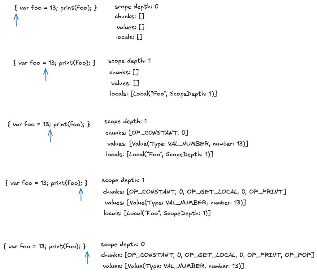
during runtime, steps in a workflow can access information about the context in which it’s running via context variables. for example, a workflow is made up of jobs and a job is made up of steps. so the steps context variable refers to information about the steps in the current run and the jobs refers to information about the job in the current run.
okay but what about the workflow? well, turns out workflow metadata like name or file path are on the global github context variable, which feels like a dumping ground for anything the github team didn’t feel like breaking out into another separate context variable. there’s repository data, github token data, workflow data, triggering events data, etc.
on the one hand, i get that this serves as a useful catchall with a name that is unlikely to collide with any newly introduced components to the actions domain. but wow i’m always forgetting what’s actually defined in it
you cannot reference your own action from a re-usable workflow
lets say u wrote an action to be reusable to other repos / projects. now you have some reusable workflows for others to use as well, but of course being the DRY minded developer you are you figured hey, why don’t i re-use my own reusable actions!
well, you can – but it’s not as easy as referencing them by some relative path in the repo. why? because when your reusable workflow is called, the working context is the context of the caller repository where your action files do not live. github essentially treats the external workflow call as if that workflow was written in the project itself. the only way to reference the action is by treating it like a third party and reference the fully qualified version repo name and tag where it will go and fetch it across the network
if you think that sounds like a release management nightmare, it is. each time you make a change to an action that’s referenced by a reusable workflow, you need to perform two releases: one release for the action and then another for the workflow referencing the action. you might think that a possible workaround might be to dynamically reference the same tag used to invoke the workflow. great idea, too bad you can’t do that.
as a third party actions creator, you’re not required to pin your dependencies
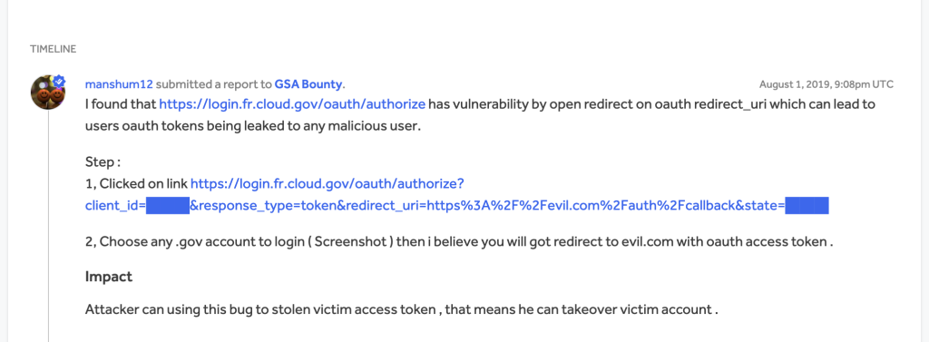
there was a security incident this year where a github actions repo was compromised and an existing tag on that repo was updated to point to a commit made by attacker that dumps out secrets. the response to this at work was to not reference action by tags which are mutable, but by sha. git even recommends this now as a security practice, but unfortunately they don’t require maintainers to pin their dependencies. so while you may be pinning the sha of an external action, that action may still be pointing to other actions by tag so you’re as safe as the weakest link.
why is it so hard to clear caches…
github offers a REST api to list and delete caches but i wish this were an option through the job view. for example, i’d like to re-run a job on my branch but from a clean cache. this appears to be available through the UI, but i haven’t been able to actually filter by branches. i don’t think this works the way they advertise it to work. either way, i really wish this were just a checkbox on the job run itself